Ultra96手に入れたので、PYNQイメージをSDに書き込みアクセラレータ試作してみた。
今回は、USBカメラで撮影した画像のヒストグラムを演算して出力する。
開発手順
1.Vivado HLSでヒストグラム演算するHW IP生成(画像読み出しとヒストグラム出力はAXI stream)
2.Vivadoで1で作ったIPと、AXI stream DMAを組み合わせてbitstream生成
3.Ultra96へJupyter Notebook経由でアクセスし、bitstreamとtclをアップロード
4.Jupyter Notebook上でUSBカメラから画像取得してIP制御するPythonコード作成
ざっとはこんな感じ。
※高位合成はするけどもやっぱりbitstream生成までが面倒。。。ここらへんSDSoC何かが良くカバーしてきていると感じるので、Pythonで一部アクセラレータをVivado HLSで作れるような仕組みがあるとおもしろいかな?
開発環境
・Vivado & Vivado HLS 2018.2
・Ultra96(PYNQ v2.3導入済み)
・USBカメラ(Logicool HD Webcam C270)
作成データ一式は以下リンク先
※bitstreamとtclとjupyternotebookをUltra96のどこかフォルダに入れてしまえば動くはず。
https://drive.google.com/drive/folders/1lxqmFfAiAzWQ6I1niS0jrUgtpuwUkTOh?usp=sharing
ヒストグラムアクセラレータのC++コード
以下のコードをVivado HLSで高位合成する。
AXI Streamのサイドチャネル制御が必要になる。
#include <stdlib.h>
#include "hls_stream.h"
#include "ap_int.h"
#include "ap_axi_sdata.h"
#define BITNUM 256
typedef hls::stream< ap_axis<32,1,1,1> > axis;
typedef unsigned int u32;
typedef unsigned char u8;
void img_hist_axis(axis &img, axis &res, u32 *height, u32 *width)
{
#pragma HLS INTERFACE s_axilite register port=return
#pragma HLS INTERFACE s_axilite register port=width
#pragma HLS INTERFACE s_axilite register port=height
#pragma HLS INTERFACE axis register both port=res
#pragma HLS INTERFACE axis register both port=img
u32 i, j;
ap_axis<32,1,1,1> tmp;
ap_axis<32,1,1,1> out;
static u32 hist[BITNUM];
#pragma HLS RESET variable=hist
for(i=0; i<*height; i++){
for(j=0; j<*width; j++){
#pragma HLS pipeline
tmp = img.read();
hist[(u8)tmp.data]++;
}
}
for(i=0; i<BITNUM; i++){
#pragma HLS pipeline
out.data = hist[i];
out.keep = tmp.keep;
out.strb = tmp.strb;
out.user = tmp.user;
out.id = tmp.id;
out.dest = tmp.dest;
if(i==BITNUM-1) out.last = 1;
else out.last = 0;
res.write(out);
}
return;
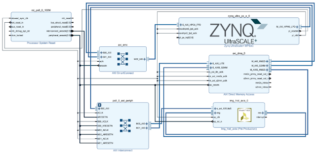
}VivadoでのHW生成
ポイントはAXI DMA経由でPSと接続するところと、AXI DMAの”Width of Buffer Length Register “をデフォルトより大きくするところ。今回は面倒なので最大値を指定(2^26)。
※画像サイズがある程度大きかったので最初この設定に気づかず、はまった。。。

Jupyter Notebookの内容
Pythonコードを貼る。
# In[1]:
from pynq import Overlay
ol = Overlay("img_hist_wrapper.bit") # Tcl is parsed here
dma = ol.axi_dma_0
img_hist = ol.img_hist_axis_0

# In[2]:
from pynq import Xlnk
import pynq.lib.dma
import numpy as np

width  = 640
height = 480

xlnk = Xlnk()
#continuous array definition for AXI Stream
image = xlnk.cma_array(shape=(height,width), dtype=np.uint32)
hist = xlnk.cma_array(shape=(256,),  dtype=np.uint32)

# In[3]:
import cv2 as cv
from PIL import Image as PIL_Image

#capturing image from USB camera
cap = cv.VideoCapture(0)
ret, frame = cap.read()
pil_img = PIL_Image.fromarray(frame)
bw_img = pil_img.resize((width, height)).convert("L")
img = np.array(bw_img)
for i in range(height):
    for j in range(width):
        image[i][j] = img[i][j]

cap.release()
bw_img #displaying captured image

# In[4]:
import time

start = time.time()
#Set the registers to IP
img_hist.write(0x10, height)
img_hist.write(0x18, width)
#Accelerator start!
img_hist.write(0x00, 1)
dma.sendchannel.transfer(image)
dma.recvchannel.transfer(hist)
dma.sendchannel.wait()
dma.recvchannel.wait()
elapsed_time = time.time() - start
print ("HW processing time:"+ str(elapsed_time*1000) + "[msec]")

# In[6]:
import matplotlib.pyplot as plt
y = hist
X = np.linspace(0, 255, 256)
plt.plot(X, y)
plt.show()

# In[7]:

start = time.time()
y, X = np.histogram(image, bins=256)
elapsed_time = time.time() - start
print ("SW processing time:"+ str(elapsed_time*1000) + "[msec]")
plt.plot(X[1:], y)
plt.show()
結果
入力画像

HW processing time:4.569292068481445[msec]
SW processing time:227.58889198303223[msec]
※SWはNumpyのヒストグラム演算
約50倍くらい高速化された!!
ちなみにヒストグラム(上がHWの結果で、下がSWの結果)比較しているとあってそうである。


コメント